Masse Feder System, Animation

In diesem Notebook wollen wir erstmal eine Simulation des Systems durchführen. Dazu benutzen wir scipy und scipy.signal.

System

Bewegungsgleichung

$M (q) \ddot{q} + g (q, \dot{q}) = Q (q)$

$[\begin{matrix} m_{1} & 0 \\ 0 & m_{2} \end{matrix}] [\begin{matrix} {\ddot{q}}_{1} \\ {\ddot{q}}_{2} \end{matrix}] + [\begin{matrix} d_{1} {\dot{q}}_{1} + d_{2} ({\dot{q}}_{1} + {\dot{q}}_{2}) + c_{1} q_{1} + c_{2} (q_{1} - q_{2}) \\ d_{3} {\dot{q}}_{2} - d_{2} ({\dot{q}}_{1} - {\dot{q}}_{2}) + c_{3} q_{2} - c_{2} (q_{1} - q_{2}) \end{matrix}] = [\begin{matrix} F_{1} \\ F_{2} \end{matrix}]$

Zustandsraum

$\dot{x} = A x + B u$

$[\begin{matrix} {\dot{x}}_{1} \\ {\dot{x}}_{2} \\ {\dot{x}}_{3} \\ {\dot{x}}_{4} \end{matrix}] = [\begin{matrix} 0 & 0 & 1 & 0 \\ 0 & 0 & 0 & 1 \\ - \frac{c_{1} + c_{2}}{m_{1}} & \frac{c_{2}}{m_{1}} & - \frac{d_{1} + d_{2}}{m_{1}} & \frac{d_{1}}{m_{1}} \\ \frac{c_{2}}{m_{2}} & - \frac{c_{2} + c_{3}}{m_{2}} & \frac{d_{2}}{m_{2}} & - \frac{d_{2} + d_{3}}{m_{2}} \end{matrix}] + [\begin{matrix} 0 & 0 \\ 0 & 0 \\ \frac{1}{m_{1}} & 0 \\ 0 & \frac{1}{m_{2}} \end{matrix}] [\begin{matrix} F_{1} \\ F_{2} \end{matrix}]$

import numpy as np
from numpy import sin, cos

import scipy.integrate as integrate
import scipy.linalg
import scipy.signal as signal
import scipy

import matplotlib.pyplot as plt
import matplotlib.patches as patches4
from matplotlib import animation, rc
from IPython.display import HTML
plt.style.use('ggplot')

m1 = 1.0
d1 = 0.1
c1 = 1.0

m2 = 1.0
d2 = 0.1
c2 = 1.0

d3 = 0.5
c3 = 1.0

def derivs(state, t, action):

    q1 = state[0]    
    q2 = state[1]
    q1d = state[2]
    q2d = state[3]

    F1 = action[0]
    F2 = action[1]

    M = np.array([[m1, 0.], [0., m2]])

    gqqd = np.array([[d1*q1d+d2*(q1d-q2d)+c1*q1+c2*(q1-q2)], [d3*q2d-d2*(q1d-q2d)+c3*q2-c2*(q1-q2)]])

    Qq = np.array([[F1],[F2]])

    M_inv = np.linalg.inv(M)
    qdd = M_inv @ (-gqqd+Qq)

    dydx = np.zeros_like(state)
    dydx[0] = q1d
    dydx[1] = q2d
    dydx[2] = qdd[0]
    dydx[3] = qdd[1]

    return dydx

# create a time array from 0..100 sampled at 0.05 second steps
dt = 0.05
t = np.arange(0.0, 20, dt)

q1 = 2.0
qd1 = 0.0

q2 = -2.0
qd2 = 0.0

# initial state
state = np.array([q1, q2, qd1, qd2])
state_0 = state

# action
action = np.array([0,0])

y = integrate.odeint(derivs, state, t, args=(action,))

q1 = y[:,0]
q2 = y[:,1]

# plot
plt.plot(t, q1)
plt.plot(t, q2)
#plt.grid()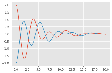

fig = plt.figure()
ax = fig.add_subplot(111, autoscale_on=False)

#ax.set_aspect('equal', 'box')
ax.axis('equal')
ax.set(xlim=(-5,5),ylim=(-5, 6))
ax.set()
#ax.grid()

patch1 = patches.Rectangle((0, 0), 1.0, 1.0, fc='k')
patch2 = patches.Rectangle((0, 0), 1.0, 1.0, fc='k')
time_template = 'time = %.1fs'
time_text = ax.text(0.05, 0.9, '', transform=ax.transAxes)

def init():
    ax.add_patch(patch1)
    ax.add_patch(patch2)
    time_text.set_text('')
    return patch1, patch2, time_text

def animate(i):
    patch1.set_x(q1[i]-0.5)
    patch2.set_x(q2[i]-0.5)
    
    time_text.set_text(time_template % (i*dt))
    return patch1, patch2, time_text

anim = animation.FuncAnimation(fig, animate, np.arange(1, len(y)),
                              interval=25, blit=True, init_func=init)

HTML(anim.to_jshtml())

Fazit

Nachdem erste Simulationen durchgeführt und die grundsätzliche Struktur des Systems durch die Modellbildung bekannt sind, müssen Systeme mit der Wirklichkeit abgeglichen werden.

In der Regelungstechnik spricht man dann von einer Grey-Box Systemidentifikation und in der Robotik von der Parameteridentifikation.