import numpy as np
from numpy import sin, cos

import scipy.integrate as integrate
import scipy.linalg
import scipy.signal as signal
import scipy

import matplotlib.pyplot as plt
import matplotlib.patches as patches
from matplotlib import animation, rc
from IPython.display import HTML
plt.style.use('ggplot')Nach dem ein mathematisches/physikalisches Modell eines mechanischen Systems zur Verfügung steht wollen wir üblicherweise erste Simulation durchführen. Bis zu einem gewissen Grad kann auch die Korrektheit des Modells überprüft werden. Zum Beispiel sollte die Schwerkraft dafür sorgen, dass das Pendel nach unten fällt (falls Reibung vorhanden).
Dieses Vorgehen hat natürlich Grenzen. Letztlich muss ein Modell immer mit Messdaten abgeglichen werden. Das erfolgt durch das bestmögliche Anpassen der Modellparameter.
Für die Simulation und Animation benötigen wir die 3 Python-Bibliotheken numpy, scipy und matplotlib.
Nichtlineares System
Nichtlineare mechanische System werden einerseits in der Form der Bewegungsgleichung oder in der Form eines Zustandsraums dargestellt.
Bewegungsgleichung
Die Bewegungsgleichung
\[ \mathbf{M}(\mathbf{q})\ddot{\mathbf{q}} + \mathbf{g}(\mathbf{q},\dot{\mathbf{q}}) = \mathbf{Q}(\mathbf{q}) \]
für das Wagen Pendel System kann aus dem letzten Blogeintrag übernommen werden und lautet
\[ \begin{bmatrix}m_{c} + m_{p} & l m_{p} \cos{\left(q_{2} \right)}\\l m_{p} \cos{\left(q_{2} \right)} & l^{2} m_{p}\end{bmatrix} \begin{pmatrix} \ddot{q}_1 \\ \ddot{q}_2 \end{pmatrix} + \begin{pmatrix}d_{c} \dot{q}_{1} - l m_{p} \dot{q}_{2}^{2} \sin{\left(q_{2} \right)}\\d_{p} \dot{q}_{2} + g l m_{p} \sin{\left(q_{2} \right)}\end{pmatrix} = \begin{pmatrix} F_c \\ 0 \end{pmatrix}. \]
Zustandsraum
Für das Lösen der Differentialgleichung ist jedoch eine Darstellung im Zustandsraum
\[ \dot{\mathbf{x}} = \mathbf{f}(\mathbf{x},\mathbf{u}) \]
geeigneter. Durch das Umstellen und Multiplizieren mit der inversen Massenmatrix \(\mathbf{M}(\mathbf{q})^{-1}\) erhalten wir
\[ \ddot{\mathbf{q}}=-\mathbf{M}(\mathbf{q})^{-1}\left(\mathbf{g}(\mathbf{q},\dot{\mathbf{q}})-\mathbf{B}(\mathbf{q}) \mathbf{u}\right) \]
für die Beschleunigung. Mit dem Zustandsvektor \(\mathbf{x}^T = \begin{pmatrix} \mathbf{x}_1 & \mathbf{x}_2 \end{pmatrix}^T = \begin{pmatrix} \mathbf{q} & \dot{\mathbf{q}} \end{pmatrix}^T\) lautet die Zustandsraumdarstellung
\[ \begin{split} \dot{\mathbf{x}} &= \begin{pmatrix} \dot{\mathbf{q}} \\ -\mathbf{M}(\mathbf{q})^{-1}\left(\mathbf{g}(\mathbf{q},\dot{\mathbf{q}}) - \mathbf{B}(\mathbf{q}) \mathbf{u}\right) \end{pmatrix} \\ &= \begin{pmatrix} \mathbf{x}_2 \\ -\mathbf{M}(\mathbf{x}_1)^{-1}\left(\mathbf{g}(\mathbf{x}_1,\mathbf{x}_2) - \mathbf{B}(\mathbf{x}_1) \mathbf{u}\right) \end{pmatrix} \\ &= \mathbf{f}(\mathbf{x},\mathbf{u}). \end{split} \]
Der Zustandsraum mechanische System kann noch weiter umgeschrieben werden, auf sogenannte AI-Systeme (Affine Input)
\[ \dot{\mathbf{x}} = \mathbf{f}(\mathbf{x}) + \mathbf{g}(\mathbf{x}) \mathbf{u}. \]
Für das Wagen Pendel System haben wir nun das Ergebnis
\[ \begin{pmatrix} \dot{x}_1 \\ \dot{x}_2 \\ \dot{x}_3 \\ \dot{x}_4 \end{pmatrix} = \begin{pmatrix}x_{3}\\x_{4}\\\frac{d_{c} x_{3} - l m_{p} x_{4}^{2} \sin{\left(x_{2} \right)}}{- m_{c} + m_{p} \cos^{2}{\left(x_{2} \right)} - m_{p}} - \frac{\left(d_{p} x_{4} + g l m_{p} \sin{\left(x_{2} \right)}\right) \cos{\left(x_{2} \right)}}{- l m_{c} + l m_{p} \cos^{2}{\left(x_{2} \right)} - l m_{p}}\\- \frac{\left(- m_{c} - m_{p}\right) \left(d_{p} x_{4} + g l m_{p} \sin{\left(x_{2} \right)}\right)}{- l^{2} m_{c} m_{p} + l^{2} m_{p}^{2} \cos^{2}{\left(x_{2} \right)} - l^{2} m_{p}^{2}} - \frac{\left(d_{c} x_{3} - l m_{p} x_{4}^{2} \sin{\left(x_{2} \right)}\right) \cos{\left(x_{2} \right)}}{- l m_{c} + l m_{p} \cos^{2}{\left(x_{2} \right)} - l m_{p}} \end{pmatrix} + \begin{pmatrix}0 \\0 \\\frac{1}{m_{c} + m_{p} \sin^{2}{\left(x_{2} \right)}} \\- \frac{\cos{\left(x_{2} \right)}}{l \left(m_{c} + m_{p} \sin^{2}{\left(x_{2} \right)}\right)} \end{pmatrix} F_c. \]
Code
mc = 1.0
mp = 1.0
dc = 0.5
dp = 0.5

l = 3.0

g = 9.81
def derivs(state, t, action):
q1 = state[0] # state 1
q2 = state[1] # state 2
q1d = state[2] # state 3, d for dot
q2d = state[3] # state 4, d for dot
Fc = action[0]
M = np.array([[mc+mp, l*mp*np.cos(q2)],
[l*mp*cos(q2), l**2*mp]])
gqqd = np.array([[-l*mp*q2d**2*np.sin(q2) + dc*q1d],
[g*l*mp*np.sin(q2) + dp*q2d]])
Qq = np.array([[Fc]])
M_inv = np.linalg.inv(M)
qdd = M_inv @ (-gqqd+Qq) # dd for ddot
dydx = np.zeros_like(state)
dydx[0] = q1d
dydx[1] = q2d
dydx[2] = qdd[0]
dydx[3] = qdd[1]
return dydx# create a time array from 0..20 sampled at 0.05 second steps
dt = 0.05
t = np.arange(0.0, 20, dt)
# initial state
x0 = 2.0
phi0 = 175 * np.pi / 180
v0 = 0.0
omega0 = 0.0
# initial state
state = np.array([x0, phi0, v0, omega0])
state_0 = state
# action
action = np.array([0])y = integrate.odeint(derivs, state, t, args=(action,))
x = y[:,0]
phi = y[:,1]
v = y[:,2]
omega = y[:,3]
r1x = x
r1y = np.ones_like(x)*0.5
r2x = l*np.sin(phi) + r1x
r2y = -l*np.cos(phi) + r1y
# plot
plt.plot(t, r1x)
plt.plot(t, r2x)
#plt.grid()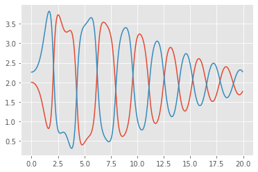
fig = plt.figure()
ax = fig.add_subplot(111, autoscale_on=False)

#ax.set_aspect('equal', 'box')
ax.axis('equal')
ax.set(xlim=(-5,15),ylim=(-5, 6))
ax.set()
#ax.grid()

line, = ax.plot([], [], 'o-', lw=2)
patch = patches.Rectangle((0, 0), 1.0, 1.0, fc='k')
time_template = 'time = %.1fs'
time_text = ax.text(0.05, 0.9, '', transform=ax.transAxes)
def init():
    ax.add_patch(patch)
    line.set_data([], [])
    time_text.set_text('')
    return patch, line, time_text
def animate(i):
thisx = [r1x[i], r2x[i]]
thisy = [r1y[i], r2y[i]]
patch.set_x(r1x[i]-0.5)
line.set_data(thisx, thisy)
time_text.set_text(time_template % (i*dt))
return patch, line, time_textanim = animation.FuncAnimation(fig, animate, np.arange(1, len(y)),
interval=25, blit=True, init_func=init)# Remark: does not work in VSCODE
# Bugfix: install ffmpeg, fix libopenh264.so.5
# HTML(anim.to_html5_video())HTML(anim.to_jshtml())Fazit
Simulation und Animation
Wir haben mit Hilfe der Methode Lagrange II das mechanische System Wagen mit mathematischem Pendel hergeleitet. Uns steht nun ein Modell zur Verfügung welches für Simulationen und Animationen verwendet werden kann.
Regelentwurf
Des Weiteren können wir dieses Modell für den Entwurf eines Reglers verwenden. Je nach Regelaufgabe stehen ein Vielzahl an Entwürfen zur Verfügung. Hier eine kurze Liste üblicher Regler für das Wagen-Pendel System:
- Zustandsregler
- LQR
- FKL
- Energiebasierte Regler
- viele mehr
KI | Maschinelles Lernen | Bestärkendes Lernen
Abschließend sei auch noch erwähnt, dass wir dieses Modell auch als Umgebung für das Bestärkende Lernen verwenden können. Liste üblicher KI-Methoden:
- Regler Gradient (Policy Gradient)
- Q-Faktor Methoden (e.g. Q-Learning)
- Modellbasierte Methoden
- viele mehr
Wir werden in zukünftigen Blogeinträgen einige Regler und KI-Methoden besprechen.