import numpy as np
from numpy import sin, cos

import scipy.integrate as integrate
import scipy.linalg
import scipy.signal as signal
import scipy

import matplotlib.pyplot as plt
import matplotlib.patches as patches
from matplotlib import animation, rc
from IPython.display import HTML
plt.style.use('ggplot')In diesem Notebook wollen wir die Parameteridentifikation besprechen wie sie oft in der Robotik durchgeführt wird.
Die Theorie der Parameteridentifikation ist innerhalb der Robotik ein eigenes Feld und durchaus weit entwickelt. Wir werden hier erstmal nur die Idee streifen und ein einfaches Beispiel lösen. In der Zukunft werden wir noch darauf zurückkommen.
Ausgangspunkt ist das physikalische Modell aus dem letzten Blogeintrag.
Physikalisches Modell
Bewegungsgleichung
Gegeben sei eine Bewegungsgleichung
\[ \mathbf{M}(\mathbf{q})\ddot{\mathbf{q}} + \mathbf{g}(\mathbf{q},\dot{\mathbf{q}}) = \mathbf{Q}(\mathbf{q}) \]
welche für das Masse Feder System mit
\[ \begin{bmatrix} m_1 & 0 \\ 0 & m_2 \end{bmatrix} \begin{bmatrix} \ddot{q}_1 \\ \ddot{q}_2 \end{bmatrix} + \begin{bmatrix} d_{1}\dot{q}_1+d_{2}(\dot{q}_1+\dot{q}_2)+c_{1}q_1+c_{2}(q_1-q_2) \\ d_{3}\dot{q}_2-d_{2}(\dot{q}_1-\dot{q}_2)+c_{3}q_2-c_{2}(q_1-q_2) \end{bmatrix} = \begin{bmatrix} F_{1} \\ F_{2} \end{bmatrix} \]
beschrieben ist. Es wird angenommen, dass zwar die Struktur der Bewegungsgleichung bekannt ist, jedoch die Parameter \(\mathbf{p} = \begin{pmatrix} m_1 & m_2 & c_1 & c_2 & c_3 & d_1 & d_2 & d_3 \end{pmatrix}^T\) unbekannt sind.
Parametergleichung für die Identifikation
Für viele mechanische Systeme kann die Bewegungsgleichung in eine Parametergleichung der Form
\[ \mathbf{H}(\mathbf{q}, \dot{\mathbf{q}}, \ddot{\mathbf{q}}) \mathbf{p}_l(\mathbf{p}) = \mathbf{h}_0(\mathbf{q}, \dot{\mathbf{q}}, \ddot{\mathbf{q}}, \mathbf{u}) \]
umgeschrieben werden. Dabei spricht man von einer nichtlinearen Messdatenmatrix oder Informationsmatrix \(\mathbf{H}(\mathbf{q}, \dot{\mathbf{q}}, \ddot{\mathbf{q}})\), einem linearen verklumpten Parametervektor \(\mathbf{p}_l(\mathbf{p})\) und einem bekannten nichtlinearen Eingangsvektor \(\mathbf{h}_0(\mathbf{q}, \dot{\mathbf{q}}, \ddot{\mathbf{q}}, \mathbf{u})\).
Für das Masse Feder System soll die Parametergleichung
\[ \begin{bmatrix} \ddot{q}_1 & 0 & \dot{q}_1 & \dot{q}_1-\dot{q}_2 & 0 & q_1 & q_1-q_2 & 0 \\ 0 & \ddot{q}_2 & 0 & -\dot{q}_1+\dot{q}_2 & \dot{q}_2 & 0 & -q_1+q_2 & q_2 \end{bmatrix} \begin{bmatrix} m_1 \\ m_2 \\ d_1 \\ d_2 \\ d_3 \\ c_1 \\ c_2 \\ c_3 \\ \end{bmatrix} = \begin{bmatrix} F_{1} \\ F_{2} \end{bmatrix} \]
lauten. Dieses Beispiel ist ein Spezialfall, da die Parameter \(\mathbf{p}_l(\mathbf{p})=\mathbf{p}\) linear in die Gleichung eingehen. Weiters sind auch die Größen \(\mathbf{H}(\mathbf{q}, \dot{\mathbf{q}}, \ddot{\mathbf{q}})\) und \(\mathbf{h}_0(\mathbf{q}, \dot{\mathbf{q}}, \ddot{\mathbf{q}}, \mathbf{u})\) linear.
m1 = 1.0
d1 = 0.1
c1 = 0.5

m2 = 0.75
d2 = 0.15
c2 = 0.75

d3 = 0.5
c3 = 1.0

p_real = np.array([[m1,m2,d1,d2,d3,c1,c2,c3]]).T
def derivs(state, t, action):
q1 = state[0]
q2 = state[1]
q1d = state[2]
q2d = state[3]
F1 = action[0]
F2 = action[1]
M = np.array([[m1, 0.], [0., m2]])
gqqd = np.array([[d1*q1d+d2*(q1d-q2d)+c1*q1+c2*(q1-q2)], [d3*q2d-d2*(q1d-q2d)+c3*q2-c2*(q1-q2)]])
Qq = np.array([[F1],[F2]])
M_inv = np.linalg.inv(M)
qdd = M_inv @ (-gqqd+Qq)
dydx = np.zeros_like(state)
dydx[0] = q1d
dydx[1] = q2d
dydx[2] = qdd[0]
dydx[3] = qdd[1]
return dydx
D = np.array([[0., 0.],[0., 0.]])# create a time array from 0..100 sampled at 0.05 second steps
dt = 0.05
t = np.arange(0.0, 20, dt)
q1 = 2.0
qd1 = 0.0
q2 = -2.0
qd2 = 0.0
# initial state
state_0 = np.array([q1, q2, qd1, qd2])
state = state_0
x = np.zeros((len(t),4))
x[0] = state_0
u1 = np.ones(len(t))
u2 = np.ones(len(t))t.shape(400,)action = np.vstack((u1,u2)).T
action.shape(400, 2)for i in range(1,len(t)):
tspan = [t[i-1],t[i]]
next_state = integrate.odeint(derivs, state, tspan, args=(action[i],))
x[i] = next_state[1]
state = next_state[1]t_ = t[1:]
q1 = x[1:,0]
q2 = x[1:,1]
qd1 = x[1:,2]
qd2 = x[1:,3]
qdd1 = (x[1:,2]-x[0:-1,2])/dt
qdd2 = (x[1:,3]-x[0:-1,3])/dt
u1 = action[1:,0]
u2 = action[1:,1]# plot
plt.plot(t_, q1)
plt.plot(t_, q2)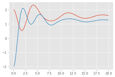
def InformationMatrix(q1,q2,qd1,qd2,qdd1,qdd2,u1,u2):
    H = np.array([[qdd1, 0, qd1, qd1-qd2, 0, q1, q1-q2, 0],[0, qdd2, 0, -qd1+qd2, qd2, 0, -q1+q2, q2]])
    h0 = np.array([[u1],[u2]])
    return H, h0
H, h0 = InformationMatrix(q1[0],q2[0],qd1[0],qd2[0],qdd1[0],qdd2[0],u1[0],u2[0])
print(H.shape)
print(h0.shape)(2, 8)
(2, 1)H = np.zeros((2*len(t_),8))
h0 = np.zeros((2*len(t_),1))H[0:2,:]array([[0., 0., 0., 0., 0., 0., 0., 0.],
[0., 0., 0., 0., 0., 0., 0., 0.]])for i in range(0,len(t_)):
H[2*i:2*i+2,:], h0[2*i:2*i+2,:] = InformationMatrix(q1[i],q2[i],qd1[i],qd2[i],qdd1[i],qdd2[i],u1[i],u2[i])p_est = np.linalg.pinv(H)@h0np.round(p_est.T,decimals=2)array([[1. , 0.74, 0.09, 0.13, 0.48, 0.5 , 0.76, 1. ]])p_real.Tarray([[1. , 0.75, 0.1 , 0.15, 0.5 , 0.5 , 0.75, 1. ]])np.round((p_real.T-p_est.T)/p_real.T*100,decimals=1)array([[ 0.3, 1.5, 13.3, 10.8, 4.8, 0.4, -1.3, -0.2]])TODO: Validierung durch neue Messdaten notwendig.
Fazit
Wir haben eine Parameteridentifikation durchgeführt wie sie oft in Robotik Büchern zu finden ist. Die Schätzung liefert gute Ergebnisse.
Die Qualität der Schätzung hängt immer von der Qualität der Messdaten ab. Die Struktur der Parametergleichung kann genutzt werden, um optimale Trajektorien für optimale Messdaten zu erzeugen. Dieses Vorgehen wurde hier nicht verfolgt.
Referenzen
- Modeling, Identification & Control of Robots (W Khalil, E Dombre)