import numpy as np
import scipy.signal as signal
import matplotlib.pyplot as plt
import scipyDas bestärkende Lernen bietet eine leicht abgewandelte Form der Regler-Iteration an.
Modellbasierte Generalisierte Offline Regler-Iteration
Aus dem letzten Blogeintrag haben wir für die Bellman Gleichung, die Lyapunov Gleichung
\[ (A-BK)^TP_{K}(A-BK)-P_{K}+Q+K^TRK = 0 \]
hergeleitet. Diese Gleichung kann iterativ
\[ P_{K}^{i+1} = (A-BK)^TP_{K}^{i}(A-BK)+Q+K^TRK \]
gelöst werden. Wird diese Iteration nicht bis zu Konvergenz durchgeführt, sondern nach einigen Schritten abgebrochen, spricht man von der generalisierten Regler-Iteration.
Hinweis
- Initialisierung: Auswahl eines zulässige (z.B., stabilisierend) Regler
\[u=K_0 x_k\]
\[P_0=0\]
- Werte Aktualisierung: Zu Zeitpunkt j, n-Schritte Iteration der Regler Evaluierung:
\[P_{j}^{i+1} = (A-BK_j)^T P_{j}^{i}(A-BK_j)+Q+K_j^{T}RK_j\]
Für \(K_j\), setzen der Ausgangsbedingung \(P_{j}^{0}=P_{j}\). Setzen der Endbedingung nach n-Schritten \(P_{j+1} = P_j^n\)
- Regler Aktualisierung
\[ K_{j+1} = (R+B^TP_{j+1}B)^{-1}B^TP_{j+1}A \]
Implementierung
m1 = 1
d1 = 0.15
c1 = 0.3

m2 = 1
d2 = 0.15
c2 = 0.3

d3 = 0.15
c3 = 0.3

A = np.array([[0., 0., 1., 0.],
              [0., 0., 0., 1.],
              [-(c1+c2)/m1, c2/m1, -(d1+d2)/m1, d2/m1],
              [c2/m2, -(c2+c3)/m2, (d2)/m2, -(d2+d3)/m2]])
B = np.array([[0., 0.], [0., 0.], [1./m1, 0.], [0., 1/m2]])
C = np.array([[1., 0., 0., 0], [0., 1., 0., 0.]])
D = np.array([[0., 0.],[0., 0.]])
sys_c = signal.StateSpace(A, B, C, D)
dt = 0.1
sys_d = sys_c.to_discrete(dt)eig_values_c = np.linalg.eigvals(sys_c.A)
eig_values_carray([-0.225+0.92161543j, -0.225-0.92161543j, -0.075+0.54256336j,
-0.075-0.54256336j])eig_values_d = np.linalg.eigvals(sys_d.A)
eig_values_darray([0.97360179+0.08998355j, 0.97360179-0.08998355j,
0.99106754+0.05382452j, 0.99106754-0.05382452j])R = np.eye(2)*1
Q = np.eye(4)*10Code: LQR Riccati Lösung
def dlqr(A,B,Q,R):
    """ Solve LQR Problem
        Returns: Controller, Valute Function, Closed Loop Eigenvalues
    """

    #first, try to solve the ricatti equation
    P = np.matrix(scipy.linalg.solve_discrete_are(A, B, Q, R))

    #compute the LQR gain
    K = np.matrix(scipy.linalg.inv(B.T@P@B+R)@(B.T@P@A))

    eigVals, eigVecs = scipy.linalg.eig(A-B@K)

    return K, P, eigVals
Code: LQR Offline Regler Iteration
def value_iteration_sub(A,B,Q,R,Kj,Pj):
    """ value update
    """

    Ac = A-B@Kj
    Qc = Q+Kj.T@R@Kj

    Pjp = Ac.T@Pj@Ac + Qc

    P = Pjp

    return P
def value_iteration(A,B,Q,R,Kj,n):
""" value update + policy improvement
"""
Pj = np.zeros(A.shape)
for j in range(0,n):
Pjp = value_iteration_sub(A,B,Q,R,Kj,Pj)
Pj = Pjp
Kjp = policy_improvement_step(A,B,R,Pjp)
Kj = Kjp
P = Pjp
K = Kjp
return K, Pdef policy_improvement_step(A,B,R,Pjp):
""" K = (R+B^T P B)^{-1}B^T P A
"""
K = np.linalg.inv(R+B.T@Pjp@B)@B.T@Pjp@A
return Kdef generalized_policy_iteration(A,B,Q,R,K0,n,m):
""" polic_evaluation + policy_improvement
"""
Pj = np.zeros(A.shape)
Kj = K0
for j in range(0,m):
# m time policy improvement step
for i in range(0,n):
# n times value iteration step
Pjp = value_iteration_sub(A,B,Q,R,Kj,Pj)
Pj = Pjp
Kj = policy_improvement_step(A,B,R,Pjp)
K = Kj
P = Pjp
return K, Pplt.plot(np.real(eig_values_d),np.imag(eig_values_d), 'gx')
draw_circle = plt.Circle((0.0, 0.0), 1.0, color='red', fill=False, linewidth=1.0)
plt.gcf().gca().add_artist(draw_circle)
plt.axis('equal')
plt.xlim(-2, 2)
plt.ylim(-2, 2)
plt.grid()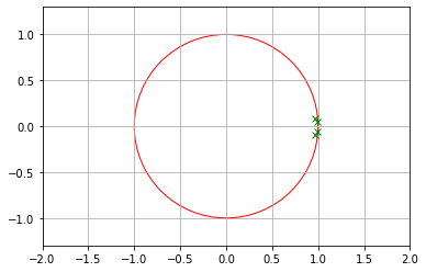
Riccati Lösung
K_infinite, P_infinite, eigVals_closed = dlqr(sys_d.A,sys_d.B,Q,R)
K_infinite
matrix([[2.09953908, 0.22634538, 3.08931627, 0.17083531],
[0.22634538, 2.09953908, 0.17083531, 3.08931627]])Regler Iteration für LQR
# Initial policy is need
Ac_eig = [0.5,0.6,0.7,0.8]
fsf1 = signal.place_poles(sys_d.A, sys_d.B, Ac_eig)
K0 = fsf1.gain_matrix
K0
array([[11.05073946, 3.76452494, 6.18886334, 0.95206432],
[ 3.76454607, 11.05330907, 0.95206947, 6.1894687 ]])K0 = fsf1.gain_matrix
n = 20
m = 20
K_j , P_j = generalized_policy_iteration(sys_d.A,sys_d.B,Q,R,K0,n,m)
print("Regler - RI Init : ", K0)
print("Regler - RI End : ", K_j)
print("Regler - Riccati : ", K_infinite)Regler - RI Init : [[11.05073946 3.76452494 6.18886334 0.95206432]
[ 3.76454607 11.05330907 0.95206947 6.1894687 ]]
Regler - RI End : [[2.09953908 0.22634538 3.08931627 0.17083531]
[0.22634538 2.09953908 0.17083531 3.08931627]]
Regler - Riccati : [[2.09953908 0.22634538 3.08931627 0.17083531]
[0.22634538 2.09953908 0.17083531 3.08931627]]print("Regler sind gleich : ", np.allclose(K_infinite,K_j))
print("Werte Funktionen sind gleich : ", np.allclose(P_infinite,P_j))Regler sind gleich : True
Werte Funktionen sind gleich : TrueFazit
Die modellbasierte generalisierte Regler Iteration zählt zu den Methoden des bestärkenden Lernens. Diese ist ein Beispiel für modellbasierte Methoden der KI. Hier haben wir eine offline generalisierte Regler-Iteration anhand des LQR Problem durchgeführt und die Lösung mit der Riccati Gleichung verglichen.